Discussion of Code Used in Prediction Model

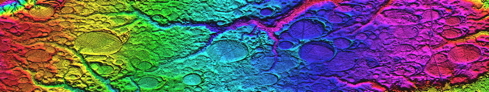
1.1 Predicting Carolina bay Orientations

1. 1.1 Predicting Carolina bay Orientations

Attempts by others at triangulation using the bays’ orientations have failed to produce a focus [Johnson, 1942]. We propose this to be caused by several large-scale geophysical flow properties not considered. First, the impact may have generated ejecta from a broad geographic extent. Secondly, a planetary body rotates during any realistic ejecta loft time. Third, the west-to-east ground-velocity between the ejection site and the landing site differs, and will be resolved as the ejecta re-enters the atmosphere and strikes the earth. Also a factor is the interpretation of a given bay’s orientation, as the bays rarely present a geometrically pure ovoid form [Eyton, J.R. and Parkhurst, J.I., 1975]. The reader should consider that generic computations for ballistic physics do not consider the resulting ground-plane velocity vector when determining a singular point-of-impact.

1.1.1 Bearing Adjustments Based on The Spherical Earth Surface

1. 1.1.1 Bearing Adjustments Based on The Spherical Earth Surface

Ejecta will follow a great circle path as it proceeds along a trajectory. For example, if an object is launched with sufficient velocity on an azimuth of 90º from latitude 45º north (i.e. due East), it will follow a great circle route as it begins to circle the earth’s surface. The Cartesian coordinate “bearing” of our example object begins to “turn” south, and eventually crosses the equator on an azimuth of 135º. During the loft period the earth would be rotating beneath the ejecta’s trajectory path; the landing location of the ejecta will actually be westward of the initial static earth target.

1.1.2 Bearing Adjustments Based on A Rotating Earth

1. 1.1.2 Bearing Adjustments Based on A Rotating Earth

Significantly, the bearing and the magnitude of the velocity vector remains the same as the “static Earth velocity vector”, rather than one derived from the geometric relationship between the impact site and the rotating-earth emplacement site. We consider that value to be the “baseline”, which is further refined in the model’s next step.

1.1.3 Bearing Adjustments Based On Latitude

1. 1.1.3 Bearing Adjustments Based On Latitude

Ground velocity differences between any two particular spots on the earth, which is a function of the cosine of the locations’ latitudes. Combining ejecta and relative ground velocity vectors causes a) atmospheric push of the ejecta and b) target drag resulting in “target contact velocity vector”, which will be rotated relative to the “static Earth velocity vector”. Figure 2 examines adjustments applied to the baseline value to generate a bearing prediction for a particular bay.

1.2 The Analytical Model

1. 1.2 The Analytical Model

We present a model for an ejecta curtain wall radiating outward from an impact site that applies geophysical flow adjustments discussed in 2.3, heuristically engineered to predict Carolina bays’ orientations. Numerical methods to evaluate ballistic trajectories at a planetary scale have been developed to generate loft distances and distribution envelopes [Jessup, K.L., et al., 2000]. While those are relevant calculations for some aspects of our study, they do not attempt to predict flow orientations at emplacement.
Our Carolina bay catalogue database spreadsheet was enhanced to generate predictions based on the spherical-earth, loft-time and latitude adjustments, generating a solution for each catalogued field’s predicted bearings while variables such as ejecta average and terminal velocity are adjusted. Charts are generated to correlate the predicted values with measured values, allowing heuristic tuning of the variables to identify best-fit solutions simultaneously across all bay fields simultaneously. The spreadsheet also generates catalogue-wide sets of GE KML to visualize in the GIS tool. The model is heuristically focused on the latitude and longitude of the proposed Saginaw crater’s three control points (NE, Centroid and SW).

1. 1.2.1 Variables

The model’s variables are segregated into those currently defaulted across all predictions (selected by best-fit solution across all evaluated bays), and those that are perturbed.
Variable:
- The Latitude and longitude of the bay location being evaluated.
Fixed:
- Crater latitude and longitude parameters (selected as
Centroid: 43.68N, 84.82W,
Rampart SW: 43.724N, 84.944W,
Rampart NE: 44.624N, 82.659W)
- A reasonable average ground-vector velocity for the ejecta as heuristically derived from our analysis. Satisfactory simultaneous solutions range from 1km/sec to 5 km/sec, with 3km/sec selected as default based on sensitivity testing)
- Three variables to generate a reasonable terminal velocity V (currently 381 m/sec) using
V = sqrt ( (2 * W) / (Cd * r * A),
where
W is droplet weight of an 1-meter diameter droplet, (in Newtons)
a density variable r (selected as 2,000 kg/meter^3) ,
and A is the frontal area of that droplet.
Cd is the Coefficient of drag of the ejecta droplet (selected as 0.3).

• - An incidence angle for ground impact to resolve ground-plane velocities (selected as 45º from vertical). The resulting ground vector of terminal velocity is 269 m/sec with the default variables.

1. 1.2.2 Loft Time Calculation and Earth Rotation Longitude Offset Value

The longitude offset calculation for a given bay location was derived mathematically based on a simple loft time to longitude relationship:
Longitude offset in degrees = Loft Time (minutes) /4
Where Loft Time = Loft Distance / Average Ground Velocity (default 3 km/sec)
The Loft Distance between the crater centroid location and that of the bay is derived using the spherical law of cosines, applied in the following Java routine. All variables in radians:

private double GreatCircleDistance(double lat1, double lon1, double lat2, double lon2) {
/* resolve distance between forePoint and farPoint input in radian
* @return The distance in Kilometres */
double dLat = (lat2 - lat1);
double dLon = (lon2 - lon1);
double a = Math.sin(dLat / 2) * Math.sin(dLat / 2) + Math.cos(lat1)
* Math.cos(lat2) * Math.sin(dLon / 2) * Math.sin(dLon / 2);
return (earthRadius * 2 * Math.atan2(Math.sqrt(a), Math.sqrt(1 - a)));}

1. 1.2.3 Determining Baseline (Static Earth) Bearing

Once determined, the model uses the longitude offset value to compute a static earth target to the east of the bay, by subtracting the offset from the bay’s longitude value. The Static Earth target site is then used to generate a baseline arrival bearing for ejecta as lofted from the impact crater’s three control points. A java routine is invoked to generate the bearing seen from [lat1, lon1] towards [lat2, lon2]. We invert the bearing 180º to create an arrival bearing. Functions convdr and convrd are used to convert between radians and degrees:

private double GreatCircleBearing(double lat1, double lon1, double lat2,
double lon2) {
double dLon = (lon2 - lon1);
double y = Math.sin(dLon) * Math.cos(lat2);
double x = Math.cos(lat1) * Math.sin(lat2) - Math.sin(lat1)
* Math.cos(lat2) * Math.cos(dLon);
double Bearing = 180 + (Math.atan2(y, x) * convrd);
return (Bearing * convdr); }

1.2.4 Applying Latitude-difference Adjustments to Base Bearing

1. 1.2.4 Applying Latitude-difference Adjustments to Base Bearing

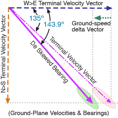
Figure 2
Figure 2 depicts the trigonometry used to adjust the arrival bearing prediction based on the latitude-driven W➔E earth ground and atmosphere rotational velocities. In our specific proposal, a relevant set of W➔E velocities would be the Saginaw crater – rotating at 1,270 km/hr – and a generic ejecta field such as Bishopville – rotating 112 km/hr faster. This ground velocity differential is combined with the terminal velocity as demonstrated as in figure 2.
We first decompose the ejecta’s terminal velocity vector (termv) to yield its W➔E component, using the base bearing ( “_C” references the centroid calculation, also done for _SW and _NE):
EWcomponent_C = termv * Math.cos(baseBearing_C) + c_deltaV;
Next, the bearing is re-composed using ACOS and the adjusted W➔E component:
componentBearing_C = Math.acos( EWcomponent_C / termv);
Finally, the bearing is cast into the proper compass quadrant (lost in the ACOS trigonometry) using the previously extracted compass quadrant of the non-rotating Earth base arrival bearing:
PredictedBearing_C = ((componentBearing_C * convrd) + (latQuadrant_C * 90));

The full Java code set includes routines to deal with compass cardinal point crossings and modulo 360º adjustments required for conversions between trigonometric notation (0º ➔ 360º) and compass bearing spherical notation (-180º ➔ +180º).

The model uses the predicted bearings to generate Google Earth kml visualization elements (paths, overlays and placemarks) for display in the GIS viewer. A sample Java routine, which generates the predicted bearing as an ”arrow” overlay, is provided here:
public String bearingArrowKML(double lat , Double lon , Double rotationValue ){
/** Returns a sting of kml to place a Bearing Arrow at a bay site given lat, lon and rotation inputs in radians **/
double distance = 2 ; /* km for building latlon box */
double NELat = Math.asin(Math.sin(lat)
* Math.cos(distance / earthRadius) + Math.cos(lat)
* Math.sin(distance / earthRadius) * Math.cos(45 * convdr));
double NELon = lon + Math.atan2(Math.sin(45 * convdr)
* Math.sin(distance / earthRadius) * Math.cos(lat),
Math.cos(distance / earthRadius) - Math.sin(lat)
* Math.sin(NELat));
double SWLat = Math.asin(Math.sin(lat)
* Math.cos(distance / earthRadius) + Math.cos(lat)
* Math.sin(distance / earthRadius) * Math.cos(225 * convdr));
double SWLon = lon Math.atan2(Math.sin(225 * convdr)
* Math.sin(distance / earthRadius) * Math.cos(lat),
Math.cos(distance / earthRadius) - Math.sin(lat)
* Math.sin(SWLat));
Double rotationValueBox = (180 -rotationValue*convrd) % 360;
final String kmlA = "";
/* elementName */
final String kmlB = "" + " " +
"Bearing Calculator V 3.0
© Cintos 2010 ]]>" +
"6" +
"http://cintos.org/ge/overlays/Bearing_Arrow.png" +
" 0.75";
final String kmlC = "";
final String kmlD = "";
final String kmlE = "";
final String kmlF = "";
final String kmlG = "";
return (kmlA + elementName + kmlB + NELat*convrd + kmlC + SWLat * convrd + kmlD + NELon * convrd + kmlE + SWLon * convrd + kmlF + rotationValueBox + kmlG);}

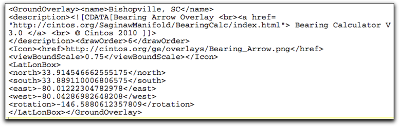
An example “GroundOverlay” kml string generated by the above routine is shown below. The example will visualize the Bishopville bearing prediction:

1. 1.3 Independent Testing of Hypothesis

To facilitate independent testing of the hypothesis, a web-based calculator is available for integration with GE. A bay’s latitude and longitude are captured using the “Placemark” kml element, which the calculator processes and generates a predicted orientation for visualization in GE. The calculator can also reverse the process, providing a “walk-back” to the putative crater by processing a user-adjusted overlay element as the input datum. Data transfers between GE and the calculator are accomplished with kml metadata.

---

Geological Research by Cintos is licensed under a Creative Commons Attribution-NonCommercial-ShareAlike 3.0 Unported License.
Based on a work at Cintos.org.
Permissions beyond the scope of this license may be available at http://cintos.org/about.html.

---

• Welcome > 
• Saginaw Manifold > 
• Bearing Calculator > 
• Code Discussion >