
Bearing Calculator For Creation of Google Earth KML to visualize Inferred bay Orientations
The kit discussed here is no longer available for public access, as Javascript is no longer supported in browsers.
All previous attempts at identifying an impact site by triangulation of the bays' inferred orientations have failed to produce a focus. We propose this to be caused by three variables not considered. First, that the impact was an oblique impact, which would infer a chaotic focus and a "butterfly" ejecta distribution. Secondly, the earth is a spherical playing field upon which Coriolis forces are a significant factor. Third, the earth rotates significantly during any realistic ejecta loft time. We characterized the spherical effects in the Systematic by Loft discussion. Earth's rotation generates west-to-east ground-velocity vectors differences between the impact site and the ejecta landing site which need to be resolved when the ejecta strikes the earth, which we discuss in the Systematic by Latitude section. If a model could be engineered to replicate those large-scale geophysical flows, it should be able to replicate the as-found orientations of all Carolina bays. Further, if the model was built to generate a distal ejecta sheet emanating from our proposed impact site, those correlations could be considered strong support for the impact argument.
Our heuristically-derived model for the distribution of ejecta from the proposed impact can be tested by generating "predicted" orientations for a given Carolina bay location, and empirically comparing that orientation to one which is apparent from that particular Carolina bay's planform. The Google Earth GIS system was leveraged to visualize numerous locations which contain Carolina bays. Using the Google Earth "Placemark" metadata element, the location's latitude and longitude are captured and annotated. A web-based calculator was developed to process those placemarks and return a set of Google Earth elements that represent the numerical model's predicted orientation. The calculator can also reverse the process, and provide a "walk-back" to a putative crater by processing a user-adjusted Bearing Arrow as the input datum. In all cases, the data transfer is accomplished by using Google Earth's "Keyhole Markup Language" (KML), a dialect of XML specifically created to encapsulate geographic information system datum.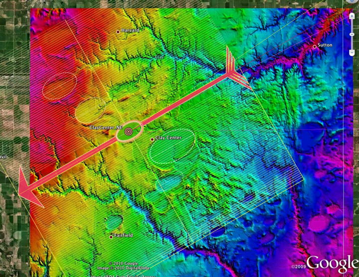
Clay Center, Nebraska Carolina bay Landforms with Calculator-Provided Predicted Bearing Arrow
Our motivation for providing the calculator as a web-based tool is to encourage testing of the relevance of the model by those interested in our conjecture. The tool must be used in concert with the freely-available Google Earth viewer. In addition to any Carolina bay location information you may already have access to, we refer the reader to two sources:
- Our growing list of individual Carolina bays - Carolina Bay Survey
These indexes will load into Google Earth desktop and iOS versions..
The great physicist John von Neumann once disposed of a mathematical argument by saying,
......"With four adjustable parameters, I can fit an elephant; with five I can wiggle his trunk."
The mathematical model developed here is considered by us to be very simple and elegant. The only variables being perturbed are the average velocity of the ejecta during its flight and the terminal velocity of the falling droplet of ejecta ( with the pellet's coefficient of drag Cd as the tuning proxy). At each field of bays, we extract the latitude and longitude as the only input variables. The model was heuristically focused on the Saginaw Bay proposed structure and it's three control points (NE, Centroid and SW); those latitude and longitude values are similarly applied as constants across all calculations. The ~200 bay location "fields" represent many tens of thousands of individual bays, and the solution sets are resolved against all fields simultaneously, with all predicted bearings falling within the control points. While it would seem plausible that the ejecta at any given location may actually have a density or velocity different from other locations, the model did not have to leverage such fine tuning to arrive at simultaneous solutions for all 200 fields.
To allow the user to interact with the model, a java web-based application was written. The "Bearing Calculator" can be driven with two different sets of data, resulting in two different types of Google Earth visualizations.
In the first case ( POINT ) the user creates a single placemark in Google Earth near a bay. That placemark is copied into the calculator and a set of elements is generated for use back inside of Google Earth. The elements identify a "Predicted" set of orientations for the site: A "bearing arrow" shows the model's prediction for an inbound bearing from the oval Saginaw craters' centroid, and two other paths predict the alignment if the ejecta had been lofted from the crater at the northerly and southerly ramparts. Note that these predict the inferred bearing as seen in the bay's alignment, not the actual bearing back the causal crater. The bearing can be generated using the second calculator use case.
In the second case [ Bearing Arrow ] the user is encouraged to adjust the bearing arrow overlay (generated in the Point case) such that it aligns with the inferred orientation of the bay or field of bays. The bearing arrow can then be copied from Google Earth and input into the calculator to generate a proposed de-skewed trajectory, which should correlate to the Saginaw crater .
The calculator defaults to an 3 kilometer/sec average trajectory speed (ground vector) and a Cd of 0.3. These values can be changed, along with the density of the ejecta and the angle of incidence of the fall.
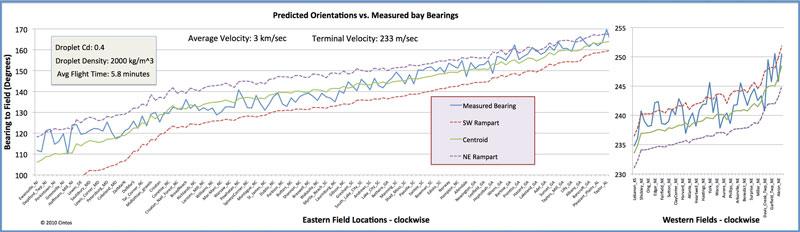
Please reference the two help pages and the calculator using the links above or the panel on the left sidebar. The chart below shows the results of the default settings, as seen at ~140 fields in the Distal Ejecta Fields kml set. The chart graphs the predicted bearing from each field assuming it had been ejected from the crater's centroid (green line) against the empirically measured inferred orientation at that field. The dashed lines represent the predicted bearing assuming the ejecta had been lofted from the northeast and southwest ramparts of the crater, and are effective control bounds for the fuzzy orientations we expect from a large impact event.
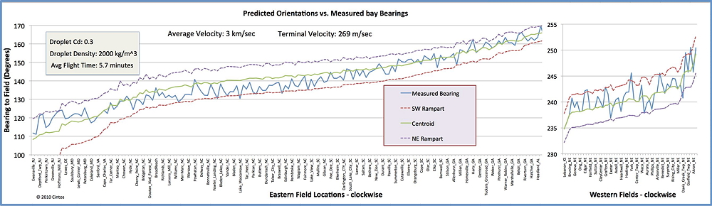
Predicted Bearings vs Measured - Image is Linked to more detailed chart.
Here is a portrait in Google Earth of how the current ~200 evaluated fields of bays correlate using the model. The kml file used to generate this display in Google Earth is available by clicking on the KMZ link Icon:
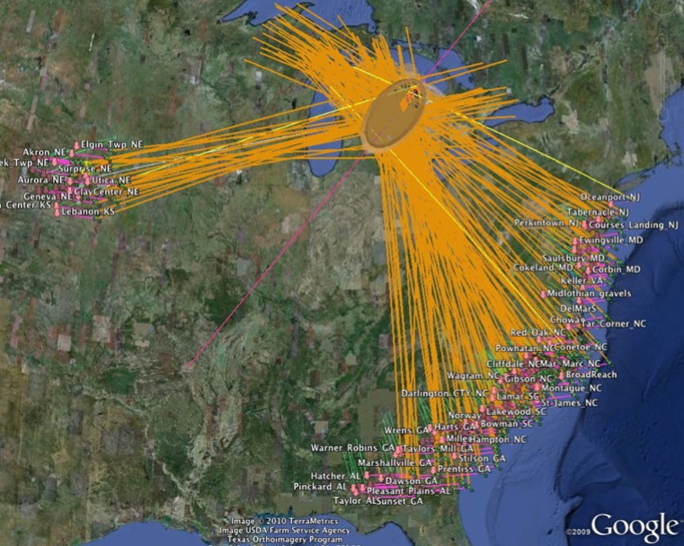
De-Skewed "Walk-Back" Model Results Displayed in Google Earth
The series of tests using both methods also generated sensitivity tests for the solutions.
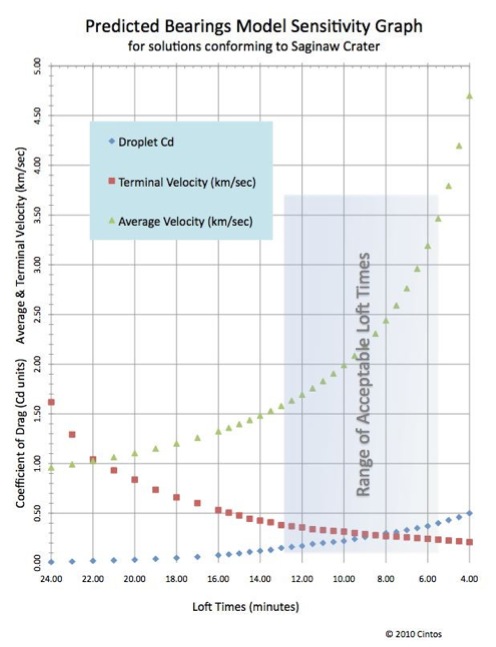
The 22-minute case represents the simplified situation where there is no atmospheric interaction, and average velocity equates to terminal velocity. Heuristically, that case was the first numerical solution developed, with only the loft time earth-rotation offset considered.
Heuristic Tuning of Variables
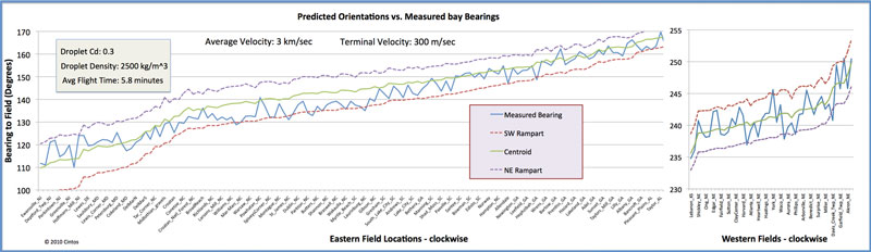
A sample of results while varying various parameters is shown below to establish the sensitivity of the tuning process to variable changes, as seen in the correlation graph. In each case, the 72 dpi jpeg image is linked to a 300 dpi TIFF version. We see the tracking of predicted values to measured values move away, either upward in bearing degrees, or downward. The effect can be balanced for good fit with sets of variables other than our current calculator default.The baseline graph uses default settings:

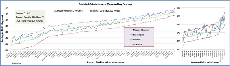
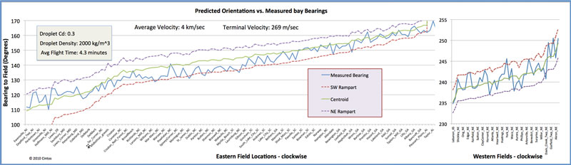
First, we perturb the Average Ground Plane Velocity from the default of 3.0 m/sec to 2.0 m/sec, then up to 4.0 m/sec:
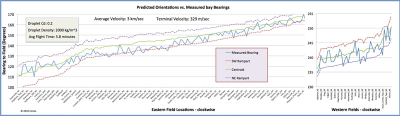
Next, we perturb the Cd value from the default of 0.3, first down to 0.2, then up to 0.4:
Finally, we perturb the Ejecta Density from the default of 2,000 kg/m^3, down to 1500 and then up to 2500:

SummaryThe authors maintain that the correlations presented here demonstrate the validity of the model’s algorithm and of our distal ejecta blanket hypothesis, and that a unique geospatial relationship exists between all known Carolina bays and the Saginaw region. Further research is proposed to investigate - in the context of our hypothesis - the geomorphological nature of Michigan’s Lower Peninsula and the Carolina bays.


Release Notes

    PredictBearings

   Version 3.0

Applet to calculate a predicted bay alignment
Input: pathBearing(  lonLat, lonLat), loft time, droplet drag coefficient, droplet density
Developed to support the Carolina bay ejecta blanket hypothesis as proposed on http://Cintos.org/SaginawManifold
2.0 - add input processing for bearing line
2.3 - Add input processing for Bearing Arrow input
2.4 - Add bearing arrow to point case output
2.5 - Use of latLon, crater and bay as case objects. Removed Line Case.
2.6 - User Interface improvements & add crater kml
2.7 - Adjust trig for proper quadrant 2 use (180º-270º), 0 & 3 not yet enabled. Add crater metrics in panel.
2.8 - Change input to average velocity vs loft time - better behaved across all loft distances
2.9 - Use surrogate crater control points & bay vs Saginaw centroid and target for better southern bearings
3.0 - Added NW quadrant math (zone 3)
Copyright 2010 by Michael Davias


Geological Research by Cintos is licensed under a Creative Commons Attribution-NonCommercial-ShareAlike 3.0 Unported License.
Based on a work at Cintos.org.
Permissions beyond the scope of this license may be available at http://cintos.org/about.html.