
Modeling of The Inferred Orientation of Carolina bays
This Section of the Saginaw Manifold discussion mirrors the posts made at the Google Earth Community Forum on Nature and Geography (Moderated)The Saginaw Impact Manifold conjecture holds that the Carolina bays structures are surface features in energetically deposited, highly hydrated, distal ejecta from a cosmic impact. A challenging aspect of the commonly proposed relationship between the bays and a cosmic impact involves the lack of an identifiable impact structure.
Most attempts at following the inferred orientation of the bays back up the trajectories' bearing have failed to produce a focus. We propose this to be caused by three variables not considered. First, that the impact may have been a "train-of-craters" event or an oblique impact, either of which would infer a chaotic focus. Secondly, the earth is a spherical playing field. Third, the earth rotates significantly during any realistic ejecta loft time. We attempt to evaluate the spherical effects in the Systematic by Loft discussion. The earth's rotation generates west-to-east ground-velocity vectors differences between the impact site and the ejecta landing site will be resolved when the ejecta strikes the earth, which we discuss in the Systematic by Latitude section.
Systematic by Loft Time
Shoot at where the target will be, not where it is right nowSystematic by Latitude
Resolve On ContactOur selection of the Saginaw Bay area of Michigan, along with the basin area westward across Michigan as a proposed impact location, allows us to revisit the loft time and trajectories of the identified Carolina bay fields. While we have leveraged the surrogate crater conceit to rationalize the inferred ejecta trajectories bearings, when we evaluate the distance covered in during the event it is appropriate to evaluate the geographic distances involved assuming a stationary earth.
Using a proposed centroid for the Saginaw Bay impact at 43.63 N latitude and 83.94 W longitude, we computed the great circle distances for each of the fields. The chart below presents the fields in a clockwise direction. We feel that the highly correlated loft distances are indicative of a common flight time, loft angle and source for the ejecta at each of the location. Note that the western fields correlate with with the eastern fields. We propose that the "butterfly" provided more energetic ejecta velocities towards the down-range direction, yielding more loft time and distance.
An oblique impact generating a butterfly ejecta distribution pattern is suggested. We have created a Google Earth overlay which, when visualized on the Google Earth facility, successfully encompasses the identified fields within two narrow bands, one to the east and one to the west.
Let us emphasize here that we fully expect the ejecta blanket to be present at distances closer and further than this "ring", but may not have been deposited on hospital terrain ( the Appalachian highlands and the Atlantic Ocean in the east and the Wisconsin Ice sheet in the west, for example).
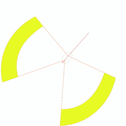
Butterfly Overlay used in Google Earth
When applied to the viewer, the following graphic is generated.
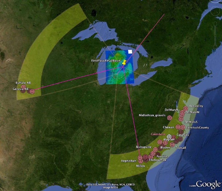
Visuialization of Butterfly Loft Range
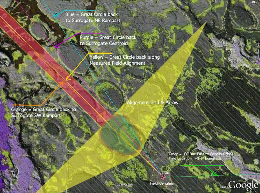
With the identification of Saginaw area as a probable impact location, our research efforts have been reinvigorated. We can now offer additional approaches to visualizing the dynamics of the impact, and to enhancing the correlations between our conjecture and the landscape. As we discussed earlier, the inferred bearing is a function of the original loft azimuth, which would have deposited the fields of ejecta out in the Atlantic Ocean (for the eastern components). An alternative to the Surrogate crater conceit is to offset the field due east by the Coriolis offset (currently 5.5 degrees), and then use trigonometric formulas to generate a great circle back along the inferred arrival bearing. The next graphic displays the Wagram field, with all the generated great circle lines identified.
The following graphic displays the Wagram field, with all the generated great circle lines identified. Many of these elements have previously been discussed and presented in earlier kml files. Our kml generator can now create sets of great circle lines emanating from a point and traveling a suggested distance along a bearing angle. For instance, the yellow line in the graphic starts at the Wagram Carolina bay field and is projected north west along the empirically derived inferred arrival bearing ( here it is ~135º). The green line at the bottom right runs due east to a point 5.5 degrees longitude east of the Wagram site. The far end of the line defines the location that this ejecta, if lofted from the Saginaw area, would have landed if the earth had not been rotating at 0.25º longitude per minute during a 22 minute loft period.
Wagram Field Local Tutorial Portrait
The next graphic displays the "tgt' as a placemark, and a great circle line segment is generated back towards the proposed crater site, again using the field's inferred arrival bearing to drive the formula.
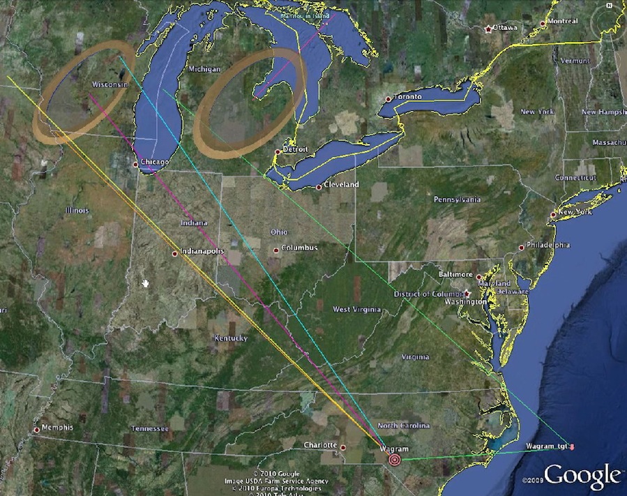
Wagram Field Trajectory Tutorial Portrait
In the above graphic, the distal ejecta is hypothetically lofted from near the south western rim of the crater, with an initial azimuth to the "Wagram Tgt" location. However, as the earth rotates west-to-east during the 22 minute loft period, the eventual landing site around Wagram in North Carolina "rolls" under the falling ejecta. The formula used to generate the great circle lines back from each the fields (both as-landed and the original Target site) is:
lat2 = asin(sin(lat1)*cos(d/R) + cos(lat1)*sin(d/R)*cos(θ))
lon2 = lon1 + atan2(sin(θ)*sin(d/R)*cos(lat1), cos(d/R)−sin(lat1)*sin(lat2))
d/R is the angular distance (in radians), where d is the distance travelled and R is the earth’s radius. θ is the inferred ejecta bearing, as empirically measured at the field.
Where lat 2, lon2 are used to create a point back along the inferred alignment bearing angle. The line is then constructed with the distal field as lat1, lon1. The length of the line (used in the formula above as d) was empirically adjusted to truncate just beyond the identified crater sites.
With this model enabled in our KML generator spreadsheet, we can very easily generate a variety of "what if" scenarios. For instance, it is very easy to regenerate the entire class of great circle lines for our ~140 ejecta fields, using a different Coriolis offset (say 28 minutes). Of course, with the empirical data available, the triangulation (especially with the inclusion of the Nebraska fields) brings forward a fairly tightly constrained loci point for the crater.
Given our new tools, it is even easier to visualize the ejecta trajectories and to reassess and reconfirm our triangulation approach. The final mash up suggest that the Saginaw Bay area is a probable impact site for distal ejecta lofted to the Carolina bay fields.
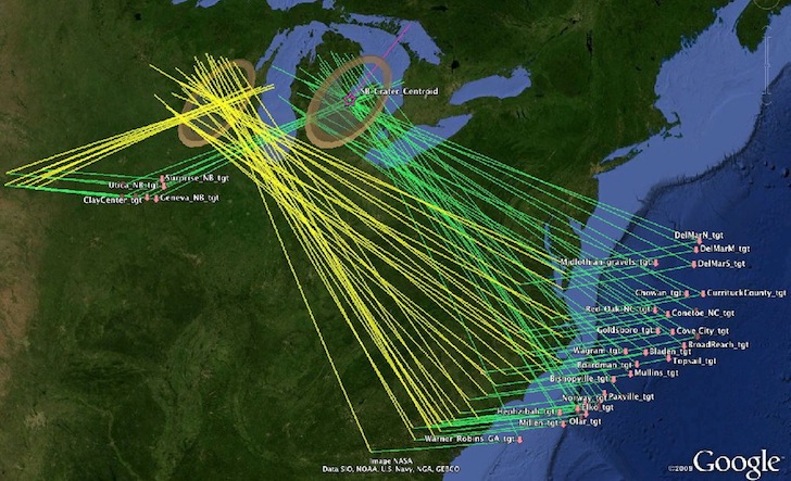
Full Set Triangualtion Great Circles - from bays to surrogate, and from pre-rotation offset bay locations toward actual site.
The solution shown in the graphic above is problematic in that the loft time is well beyond times generated by ballistic trajectory tools. Using a numerical model developed to account for the skewing of the inferred alignments during the aerodynamic breaking and landing events due to earth-rotational velocity differences which are latitude related, we now have a satisfactory solution that yields loft time in the range of 5 to 10 minutes, We discuss this "systematic by latitude" alignment factor in the subtopic page. Satisfactory results are now available with loft times in the range of 5 to 10 minutes. The following graphics show the correlation of each bay field's alignment with the proposed Saginaw impact crater .
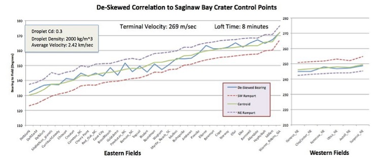
The model in use can generate correlations directly against an empirically measured bearing deskewed back to the proposed Saginaw crater location, as above, or by starting with a single point (lat, lon) and generating predicted bearing sets which we compare visually against a bay at that location. The series of tests using both methods also generated sensitivity tests for the solutions. The only variables are the loft time and the terminal velocity ( as a function of density and Cd). As shown in the figure below, the most acceptable solutions are found with a terminal velocity (in the ground plane) of 200 - 300 m/sec. We find this correlation to be highly supportive of the model's validity.
The Model
The mathematical model developed here is considered by us to be very simple and elegant. The only variables being perturbed are the average velocity of the ejecta during its flight (with loft time as the tuning proxy) and the terminal velocity of the falling droplet of ejecta ( with the pellet's coefficient of drag Cd as the tuning proxy). At each field of bays, we extract the latitude and longitude as test case input constants. The model was heuristically focused on the Saginaw Bay proposed structure and it's three control points (NE, Centroid and SW); those latitude and longitude values are similarly applied as constants across all calculations. The 42 bay location "fields" represent many thousands of individual bays, and the solution sets are resolved against all fields simultaneously, with all bearings falling within the control points. While it would seem plausible that the ejecta at any given location may actually have a density or velocity different from other locations, the model did not have to leverage such fine tuning to arrive at simultaneous solutions for all 42 fields.The great physicist John von Neumann once disposed of a mathematical argument by saying, "With four adjustable parameters, I can fit an elephant; with five I can wiggle his trunk."
Coriolis Force at work in large-scale geophysical flows
We suggest the reader reference an in-depth discussion of the Coriolis force at work in large-scale, geophysical flows, by James F. Price, Woods Hole Oceanographic Institution • an essay on the Coriolis force
Coriolis Force
See the accompanying sub-section page at Wikipedia, the free encyclopedia
Great Circle routes vs Rhumbar. GE does paths as great circle, while overlays are placed as Mercator projections, which lines show up as Rumbars.
The equation of motion for a rotating coordinate system has two terms to accommodate the rotation of the coordinate system, the centrifugal term and the Coriolis term. Generally the centrifugal term is much larger than the Coriolis term. The earth does not rotate fast enough for the centrifugal term to "throw off" an object from its's surface, it is leveraged in practical use in the case of launching spacecraft: Launching sites closer to the equator are more favorable.
The explanation of this phenomenon is mainly kinematic, i.e., more mathematical than physical.
Coriolis Force and Projectiles (
excerpt here)Federation of American Scientists, 1725 DeSales Street, NW, 6th Floor,Washington, DC 20036 , email: fas@fas.org
Projectiles which travel great distances are subject to the Coriolis force. This is a artifact of the earth's rotation. The local frame of reference (north, east, south and west) must rotate as the earth does. The amount of rotation, also known as the earth rate is dependent on the latitude: earth rate = (2p radians)/(24 hours) sin(latitude). For example, at 30o N, the earth rate is 0.13 radians/hr (3.6 x 10⁻⁵ rad/sec). As the frame of reference moves under the projectile which is traveling in a straight line, it appears to be deflected in a direction opposite to the rotation of the frame of reference.
Figure 12. Coriolis force.
In the northern hemisphere, the trajectory will be deflected to the right. A projectile traveling 1000 m/s due north at latitude 30o N would be accelerated to the right at 0.07 m/s2. For a 30 second time-of-flight, corresponding to about 30 km total distance traveled, the projectile would be deflected by about 60 m. So for long range artillery, the Coriolis correction is quite important. On the other hand, for bullets and water going down the drain, it is insignificant!
-------------------
The angular velocity of earth is 4.17 x 10^-3 deg/sec.
That is 7.27 x 10^-5 sec^-1 (1 deg ~ 0.0175 rad).
If I fire East for example, I'd be at 90 deg to the axis of the earth. But firing NE, I'd have components of both.... If I do have multiple vectors, how do I figure the effects?
Simply split velocity into "north" (angle to Earth's axis depending on latitude) and "east" (always 90 deg to axis) components, and compute and work with Coriollis forces for both. You can do this because vector product is distributive, i.e. (\vec{v}_{north}} + \vec{v}_{east}) \times \omega = \vec{v}_{north}} \times \omega + \vec{v}_{east}} \times \omega.
The "north" force component will push sideways (to east if you fire north, to west if you fire south), and the "east" component will push upwards (that's why they like to blast off eastbound near equator).
-------------------
Chusslove Illich (Часлав Илић)

Geological Research by Cintos is licensed under a Creative Commons Attribution-NonCommercial-ShareAlike 3.0 Unported License.
Based on a work at Cintos.org.
Permissions beyond the scope of this license may be available at http://cintos.org/about.html.