


Carolina Bay Survey of Individual Bay Planforms
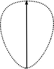
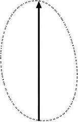
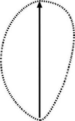
Attempts to measure the inferred alignment of the Carolina bays requires quite a lot of "interpretation", as it were. It has been recognized that the bays are not truly ovals, but seen as ovoids or ellipses. Certainly the crisp shapes of the Carolinas are standardized enough to build a shape that represents them. An overlay in this "prototype" shape would make it a bit easier to grab an orientation reference. In a process similar to the "Bearing Arrow", which is used to find the relative orientation of a field of bays, I now utilize "bay Prototype" overlays to capture individual bay planform metrics.
Maryland- New Jersey.................Classic Carolina...................Georgia, Alabama.......................Western
This shape was generated using a graphic program, and tracing from numerous bays to get a good rendition of the typical North and South Carolina bay planform. It is shown here rotated clockwise 90º for space consideration on the page here. A Java program is being developed to process these overlays. The goal will be to capture the ranges of sizes and orientation of bays within a given field. A beta version is available on the Bay Planform Survey Tool page. The calculator's output is in tab-delimited fields, for import into a spreadsheet for additional manipulation. On goal is to build a histogram of bay sizes, for comparison to generic bubble-field distributions done in other realms.
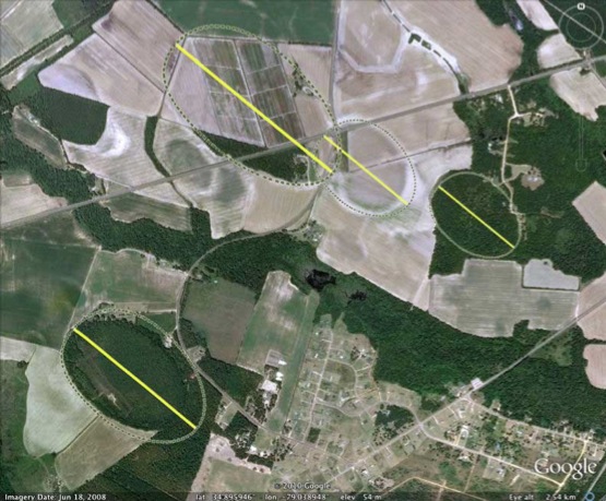
The actual image is a transparent .PNG file. Here is an example of the overlay when used in Google Earth.
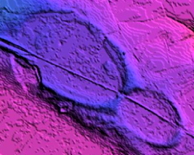
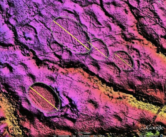
As you likely know, the imaging of bays has been enhanced by using LiDAR imagery. I have discovered a neat trick: if I create a set of image KMZ using Global Mapper, and then manually remove the highest resolution image level, I accomplish two things. First the file size is reduced substantially, allowing for quicker loading. (Some resolution is certainly lost, but for my purposes, that the finest level imagery was not all that useful). The second thing the removal does is create a situation where zooming in closer to the earth will eventually drop the LiDAR imagery out, allowing the underlying Google Earth standard imagery to be revealed. The result is the ability to simply rock back and forth between the LiDAR version of the landscape, and the visual version. For example, here is the area show above, backed out a bit, and bringing the LiDAR image into view:
I must say that this "shape" really does capture the general bay planform to a high degree of fidelity. Feel free to open the attached KMZ file and use Google Earth to create additional copies of the overlay. Click on one in the DOM and "copy/Paste" for a new instance, Then use the edit functions (or "get info") to move it over a different bay. After using the handles to rotate and resize, you will likely find it is a neat fit. Using this process, I hope to capture every bay across several "fields".
My ejecta proposal would suggest that the bay's distorted oval is a momentum artifact due to the Earth's rotational speed when the ejecta strikes the land. It remains to be determined just what the actual arrival bearing would lay, given the shape. My estimate - the yellow line - could be off by many degrees.
Adding to the post here: I have completed the first Bay Survey, identifying and capturing ~500 bays across a field of 520 square km in central SC. Two graphs are included here. The first one plots the size distribution of bays as a histogram, with one Hectare per bin. The second plots the length-width ratio of the ovoid bay planform against the area of the bay.
The KMZ file containing the LiDAR link and the individual bay overlays for "SC_Survey_B" is Available HERE.
These metrics need to be generated for (potentially) all 250 "fields" of bays in the field catalogue . Should anyone be in a position to lend a hand, I'd love to discuss a collaboration.
Our survey of Carolina bay landforms has been carried out thus far using a "field-based" approach, with the count of fields approaching 250. These can be viewed using the Distal_Ejecta_Fields.kml file. These fields are randomly sized, done in an attempt to keep their sizes down to the absolute minimum, especially when the 1-9 arc-second data is used. But the random sizes are presenting challenges as we attempt to count all the bays...
Most of the larger field DEM files have been recently further reduced by removing the tiles for the highest resolution, as they do not seem to have any additional information. It also allows for the user experience of toggling the DEM image off when zooming in very close to the earth - which then allows for viewing of the Google Earth imagery for comparison purposes.
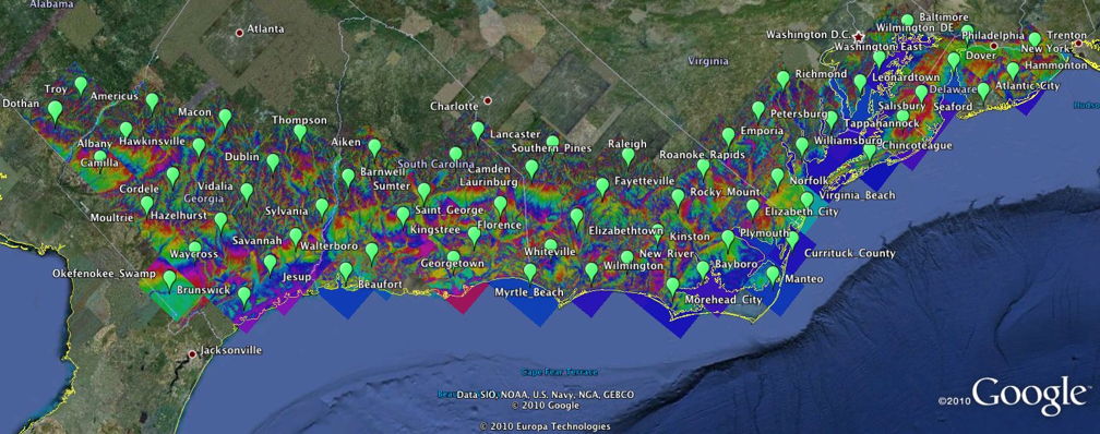
To support an ongoing effort aimed at cataloguing all the visible Carolina bays, I have generated a set of HSV-shaded DEMs using the USGS's 100k index and 1/3 arc-second data. Each of the resulting tile sets are 1º of longitude in width, and 0.5º of latitude in height. By using a fixed-size regional view, perhaps we can correlate the differences seen in each of these areas. (OK, the areas are actually different areas as we move north to south due to Earth's curvature, but close enough...) A network-linked KML element for this new 100K Quadrant index is attached to the post. In addition, the html-based Google Earth Plug-in LiDAR browser has been updated to include a "100K Quad Index" button.
Here is a graphic showing the extent of our current Eastern Index: Our undertaking is being indexed by a new set of ‘100K” USGS Quadrants. Using these fixed areas, a more structured set of metics will be obtained.
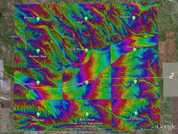
And here is the graphic for the Nebraska area

Geological Research by Cintos is licensed under a Creative Commons Attribution-NonCommercial-ShareAlike 3.0 Unported License.
Based on a work at Cintos.org.
Permissions beyond the scope of this license may be available at http://cintos.org/about.html.